Subsections of Modes
GIS Editor
Map Mode
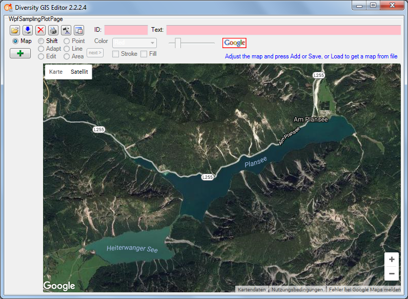
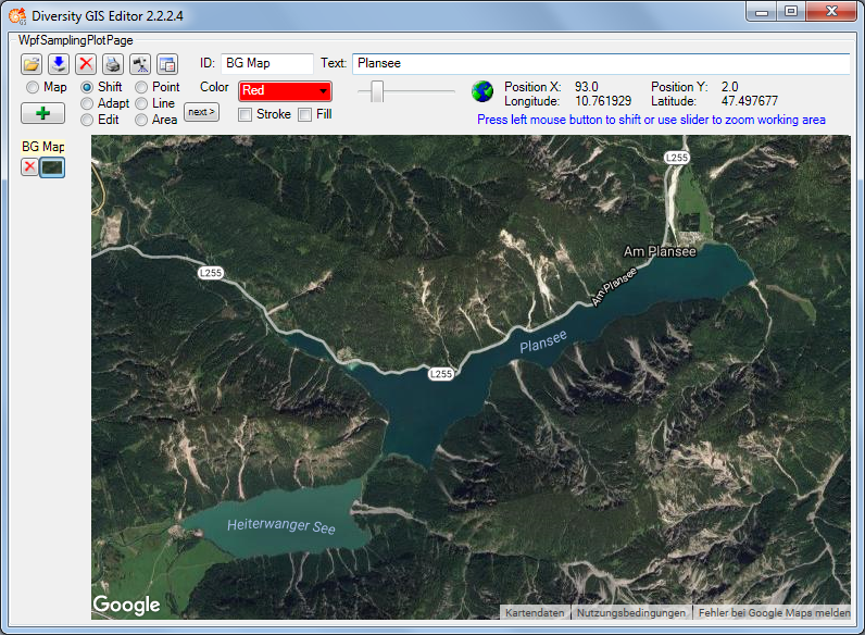
In Map mode the editor connects via Internet to the SNSB Google Maps
service or alternatively to the Open Street Maps service, regarding on
the GIS-Editor Settings, and displays an online
map which can be moved, zoomed and switched as usual. The status area
shows the  or
respectively the
or
respectively the
 symbol. The
size of the map area adapts to the size of the working area, even when
resizing the window.
symbol. The
size of the map area adapts to the size of the working area, even when
resizing the window.
In case of Google the controls for moving, zooming and map type are
displayed by default. The overview window in the bottom right corner can
be switched manually. The map can be adjusted to the user’s needs as
follows:
- Select map area: Press and hold left mouse button and move the mouse
- Zoom map: Turn the mouse wheel (if any), double click (left or right
mouse button) on a location
- Switch map type: Use Google map type control
- Hide Google controls: Click right mouse button to hide, left mouse
button to show them again
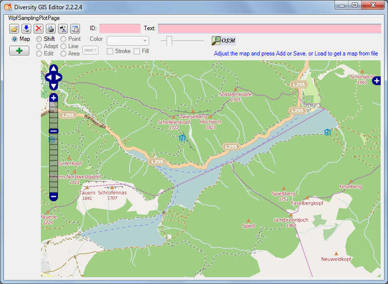
In case of Open Street Maps the pan and zoom control is displayed by
default. It can be switched off or on by clicking the left mouse button
anywhere within the map area. The layer switch control is hidden and can
be opened by pressing the  or closed
again by pressing the
or closed
again by pressing the  button on the
right side. The map can be adjusted to the user’s needs as follows:
button on the
right side. The map can be adjusted to the user’s needs as follows:
- Select map area: Press and hold left mouse button and move the mouse,
or use the OSM pan control
- Zoom map: Turn the mouse wheel (if any), double click (left mouse
button) on a location or use the OSM zoom control
- Switch map type: Open the layer switch and select a layer
- Hide or show pan and zoom control: Click left mouse button to toggle
the control
If an appropriate area has been selected, just press the Add button
 , then the area will be scanned and added to
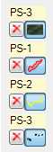
the Sample List as a reference map. A little image of the map will
appear on the toggle button in the Sample List. The controls should be
switched off before adding to get a neat map image.
, then the area will be scanned and added to
the Sample List as a reference map. A little image of the map will
appear on the toggle button in the Sample List. The controls should be
switched off before adding to get a neat map image.
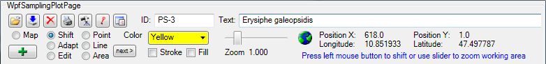
Then the mode will be switched to Shift mode automatically and the
status symbol will change to
 indicating
that world coordinates are present. The screen and world coordinates
will be shown in the status lines if the mouse is moved over the map
surface.
indicating
that world coordinates are present. The screen and world coordinates
will be shown in the status lines if the mouse is moved over the map
surface.
The maps are subject to the Mercator projection, which is the GIS
Editor’s precondition for every bitmap used as a reference map. While
the screen coordinates are linear in horizontal and vertical direction,
the world coordinates are non linear in vertical direction.
GIS Editor
Shift Mode
This is the quasi default mode of the GIS Editor. The cursor changes to
a move shape  when touching the
background map. The map is “frozen” and exists as an image sample on the
sample list. Changing the map region or resolution is no longer
possible. But the Shift Mode provides 2 features:
when touching the
background map. The map is “frozen” and exists as an image sample on the
sample list. Changing the map region or resolution is no longer
possible. But the Shift Mode provides 2 features:
- Move the working area
- Zoom the working area
Moving the working area
Press and hold the left mouse button and move the mouse to shift the
working area within the display window. This is useful when having
loaded a map from a storage unit which is larger than the GIS Editor’s
window, or in combination with zooming the working area.
Zooming the working area
Place the mouse cursor at the slider control, press and hold the left
mouse button and move the control left to zoom out or right to zoom in
the working area. The range of the zoom is from factor 0.6 to 3.0. The
current value is displayed beneath the zoom control. Double click the
slider control to reset the zoom to default value 1.0.
Enlarging the working area makes it more easy to place objects
precisely. The relevant area then could be selected by moving the zoomed
working area. Downsizing the working area gives an overview of large map
regions.
Note that the resolution of the map itself does not change any more when
zooming in. But objects on the map are created in vector graphics, so
the markers, lines or areas will remain sharp and clear while zooming.
And they will adapt there thickness smoothly to the size.
GIS Editor
Area Mode
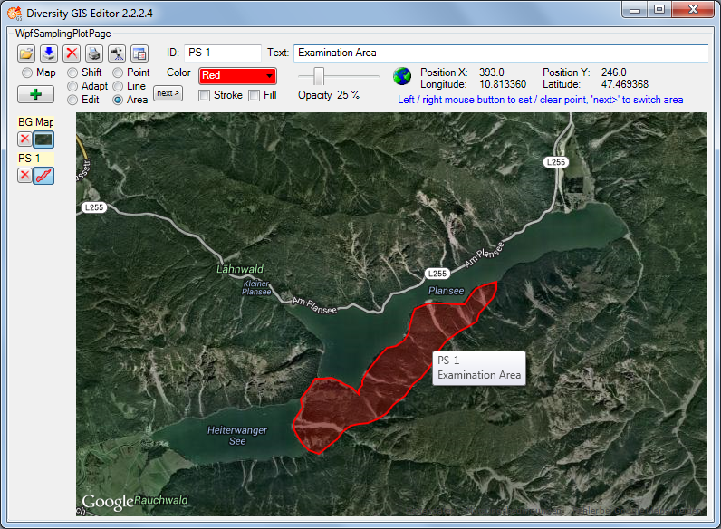
This mode is used to create areas (polygons) on the background map. The
cursor changes to a cross line when touching the background map. Each
click on the left mouse button sets a new point of the polygon. Every
click on the right mouse button clears the last point set. The closed
polygon defined by the points is displayed completely at any time. When
holding the left mouse button the point can be placed while the lines of
the polygon are shown as a “rubber band” display.
To create more than one area for a sample, just click the
 button. This will finish the current
polygon and start another one. It could be repeated without limitation
of the number of polygons.
button. This will finish the current
polygon and start another one. It could be repeated without limitation
of the number of polygons.
Setting the color
The areas are created as filled polygons, this means they have a border
line (stroke) and a filling. The color of stroke and filling can be set
independently or simultaneously by clicking the appropriate check boxes
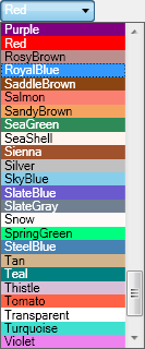
beneath the Color list box. Clicking on the list box will open a drop
down menu with the complete set of 141 predefined brushes. Use the
scroll bar to navigate to the preferred color and select it with the
left mouse button.
Setting the transparency
Besides the color the transparency of the area could also be set for
stroke and filling. In each edit mode the slider control is used for
that. The area stroke or filling changes smoothly from invisible at the
left till completely opaque on the right slider position. The value
beneath the slider control indicates the opaqueness in a range from 0%
to 100%. The default settings are 100% for stroke and 25% for filling.
Before adding the polygon to the Sample List an Identifier (ID) and a
Description (Text) should be written to the text boxes in the control
panel.
Clicking the Add button will put the
current area(s) as one sample into the Sample List. The toggle button
will show a small picture of the first area of the sample. The ID will
be displayed above the button. Furthermore a tool tip will be created
for the sample holding the ID and Description, which will pop up when
moving the mouse over the toggle button or over the polygon in the
working area.
GIS Editor
Line Mode
This mode is used to create line strings on the background map. The
usage is adequate to the Area Mode. The cursor
changes to a cross line when touching the background map. The points of
the line strings can be set or cleared by clicking the mouse buttons.
Clicking the button will switch to the
next line string for the sample. The distance of the last drawn line
string section is displayed beneath the status area.
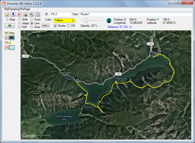
Color and transparency can be set for the line strings using the
appropriate controls, but only for stroke, because the line strings do
not have a filling. Thus checking the Fill box will have no effect.
After adding the lines to the sample list a small picture of the first
line string will appear on the toggle button.
GIS Editor
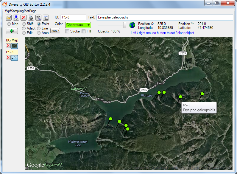
Point Mode
This mode is used to create Points (object markers) on the background
map. The usage is similar to the Area Mode. The
cursor changes to a cross line when touching the background map. The
object markers can be set by clicking the left mouse button, clicking
the right mouse button will clear the last markers one by one again. The
button has no impact, because each Point
represents a complete object and needs not to be finished before
creating the next one.
The shape of the object markers can be selected from a number of
predefined Point symbols and icons within the Settingswindow, e.g.:
|
|
| Pin: |
 |
| Diamond: |
 |
| Needle: |
 |
| Cross: |
 |
| Pyramid: |
 |
| X: |
 |
| Cone: |
 |
| Square: |
 |
| Questionmark: |
 |
| Circle: |
 |
| Minus: |
 |
| Myxomycete: |
 |
| Fungus: |
 |
| Lichen: |
 |
| Bryophyt: |
 |
| Plant: |
 |
| Evertebrate: |
 |
| Mollusc: |
 |
| Assel: |
 |
| Insect: |
 |
| Echinoderm: |
 |
| Vertebrate: |
 |
| Fish: |
 |
| Reptile: |
 |
| Bird: |
 |
| Mammal: |
 |
Color can be set for the symbol markers using the appropriate controls.
It depends on the selected point symbol, whether it just has a stroke
(e.g. “Cross”) or also a filling (e.g. “Pin”). Transparency can be set
for both, the symbol and icon markers. The stroke thickness and the size
of the markers can be set in the Settings menu.
After adding the object markers to the sample list a small picture of
the collection will appear on the toggle button.
GIS Editor
Edit Mode
This mode is used to modify all samples (objects and images) which are
currently visible on the working area. It applies to the elements of
the Sample List as well as to the current sample.
Changing the position or shape of objects (points, line strings, areas)
To change an object one has to move the vertices (“corner points”) which
are defining it. To do so just move the mouse close to a vertex to
localize it. As soon as the corner has been grabbed the cursor changes
its shape to a hand symbol  .
.
Now press the left mouse button and hold it, then move the mouse to
change the position of the vertex accordingly. The shape of the object
or the marker will change in the same manner. Release the mouse button
when the preferred position has been set.
Note that areas and line strings cannot be moved in total while keeping
their shapes!
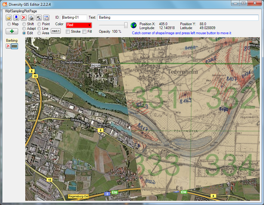
Changing the position or shape of images (maps)
Images (e.g. maps) can be moved completely (keeping their aspect ratio),
scaled in horizontal and vertical direction and skewed within an affine
transformation. Editing an image can be divided into 4 stages by
grabbing and moving the following corners:
- Top-left: Moving the total image by keeping its aspect ratio
- Bottom-right: Squeezing or stretching the image horizontally and
vertically
- Bottom-left, top-right: Skewing the image in an affine way by
keeping the corner points top-left and bottom-right at its positions
- Bottom-right again: Skewing the image in an affine way by keeping
the corner points top-left and bottom-left at its positions
Stages 1 to 4:
Changing color and transparency
Color and transparency can be set independently (or simultaneously) for
the objects using the appropriate controls and check boxes for Stroke or
Fill. The setting will affect all visible objects, so objects which
should not be changed have to be switched off before with their toggle
buttons. The color of images could not be changed, of course, but the
transparency can be set if the Fill box is checked. The transparency of
the background map cannot be changed.
GIS Editor
Adapt Mode
Essential for visualizing Geographical Objects is a background map with
world coordinates. The GIS Editor’s Map mode offers a convenient way to
create such a map, but it is restricted for the use of Google or OSM
maps which are present in the web and are providing world coordinates.
It would be nice to load scans of e.g. topographical or even historical
maps into the working area and use them as background maps, but the
problem is how to assign world coordinates to them.
The Adapt mode solves this in an easy way by executing the following
steps. As a precondition a background map having world coordinates (e.g.
a Google map) must be present which covers the area of interest of the
new map to be referenced.
-
Load the new map image using the Load button
 . The image will be placed top
left inside the working area.
. The image will be placed top
left inside the working area.
-
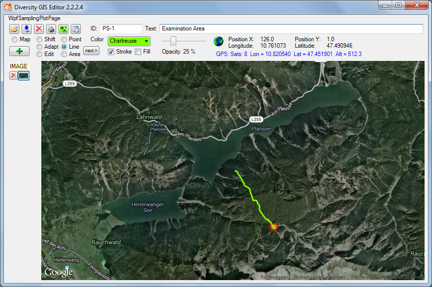
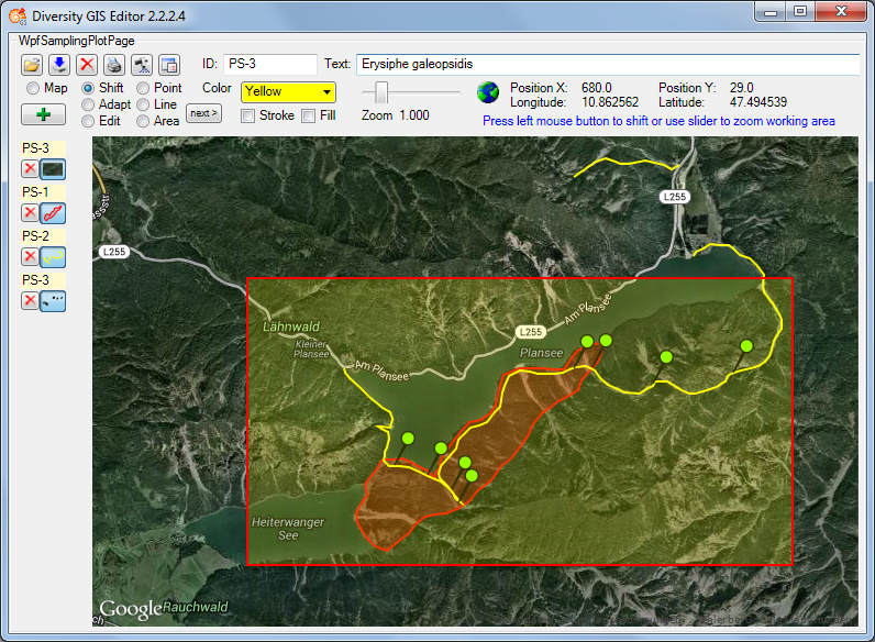
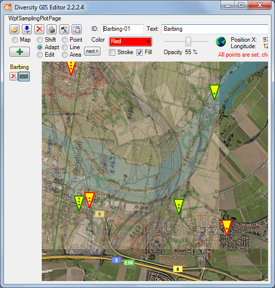
Select Adapt mode by checking the Adapt radio button. The cursor
changes to a pointer symbol  having a green border when touching the new image and having a red
one when touching the background map.
having a green border when touching the new image and having a red
one when touching the background map.
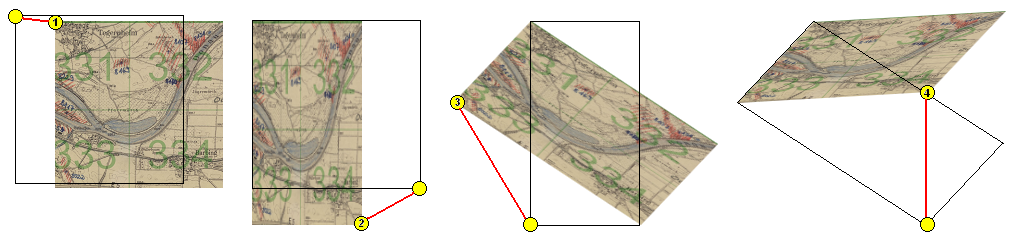
-
Now 3 reference points must be set alternately on background and new
map to assign the appropriate locations (e.g. distinctive landmarks
like road crossings). The last point can be modified as long as the
map is not changed. The cursor always tells you what reference point
will be set, according to its color and the number of dots in the
middle:


Note: It is reasonable to select distant points close to the edges
of the new map, because this will give more accurate results.
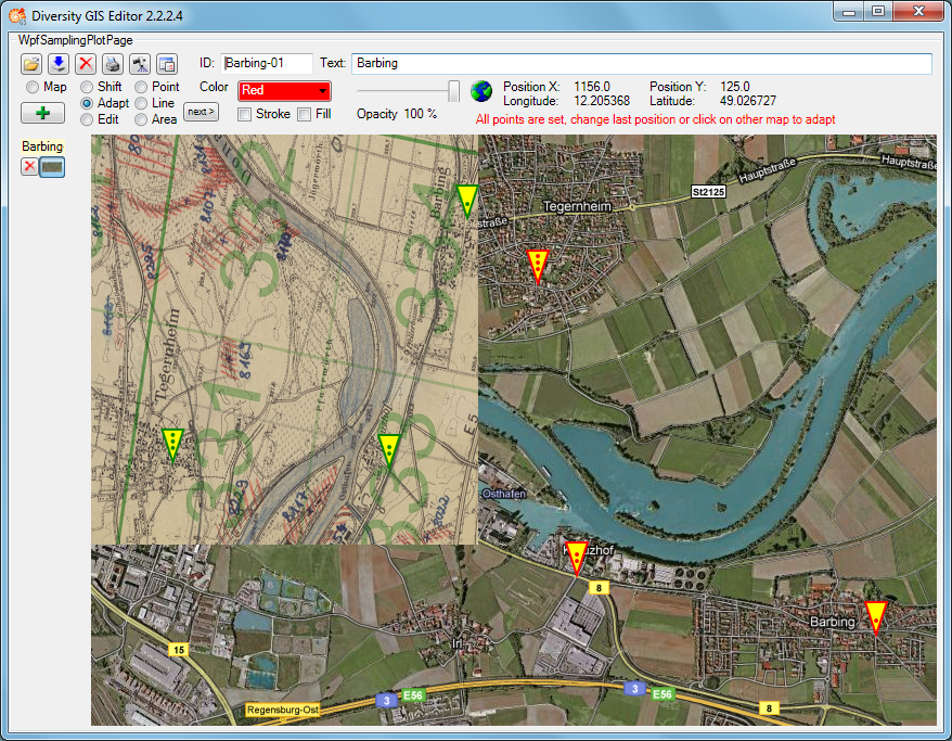
-
When all reference points have been set and the cursor touches the
alternate map, it changes to the finished shape
 . The next click will place
the new map into the appropriate background map area.
. The next click will place
the new map into the appropriate background map area.
The adapted image has been transformed to fit into the current world
coordinates of the background map. Now the new map can be added to the
sample list by pressing the Add button .
When it is finally saved to disk by pressing the Save button
 , the new assigned world coordinates will
be saved, too, in an XML file with the same name (see SaveSamples).
, the new assigned world coordinates will
be saved, too, in an XML file with the same name (see SaveSamples).
Sometimes it is difficult to place the new map and the reference map
side by side, because the window is too small, and zooming out would
blur the details needed for setting the reference points. If the new map
covers the background map, the reference points can be set anyway
Note: The Fill box must be checked to change the transparency of the
new map. The background map’s transparency cannot be changed.
Subsections of Samples
GIS Editor
Load Samples
A background map is required before objects (areas, line strings,
points) can be loaded. If no background map is available, the GIS Editor
will extract the appropriate area from the sample file data and
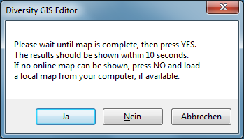
automatically adjust the map viewer to cover the region. The user is
prompted to wait until the map has been established completely and then
press  . If no map is displayed (e.g.
because there is no internet connection), the user may press
. If no map is displayed (e.g.
because there is no internet connection), the user may press
 and load a local map instead, or
 to cancel the loading of the
shapes.
to cancel the loading of the
shapes.
When loading a shape file, the objects will be displayed at the
background map according to their coordinates and added to the Sample
List automatically. The GIS Editor is able to read MS-SQL Geo Object
files (.shp1), TAB separated text files (.shp2), GPS Exchange Format
files (.gpx) as well as ArcView Shape Files (.shp).
The assumption of the type of input file is made according to the
extension of the file, so e. g. a TAB separated input file of an
external source might have to be renamed to .shp2 before it is loaded by
the GIS Editor. The input parameters of the first text line are
determined, a dialog window will open and show them on the left.
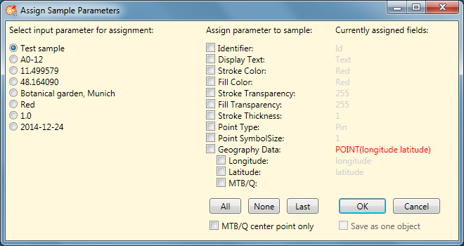
Then you have to assign certain input values to the GIS Editor
attributes, wich are displayed in the middle of the window. Select an
input parameter using the radio button on the left, then assign it to
one or more sample attributes by clicking the appropriate checkbox in
the middle. The assigned values are shown on the right side of the
window. Values in gray are default parameters, which are used if the
attribute has not been assigned. There is just one mandatory attribute
which has to be set, the Geography Data (SQL Geo Object). If there is no
SQL Geo Object available in the input file, a point object will be
created automatically when assigning longitude and latitude parameters.
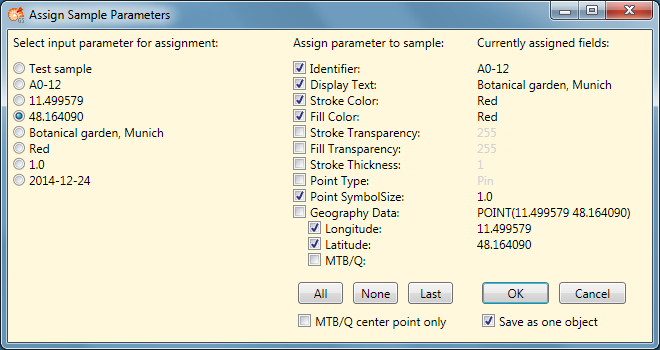
To assign up to 10 input parameters simultaneously to the adjacent 10
sample attributes, just click on the  button.
This is helpful if the input file has been created with the GIS Editor
itself, so the input values are already in the right order.
button.
This is helpful if the input file has been created with the GIS Editor
itself, so the input values are already in the right order.
To remove all assigned values, click on the  button.
If the assignment is done, click on the  button
to show all geographic objects of the input file according to the
assigned parameters. Each object will be added to the list as a separate
sample. To put all objects together as one single sample, check the
“Save as one object” box.
button
to show all geographic objects of the input file according to the
assigned parameters. Each object will be added to the list as a separate
sample. To put all objects together as one single sample, check the
“Save as one object” box.
Click on the  button to cancel the load
operation.
button to cancel the load
operation.
The last assignment is saved by the GIS Editor and can be used for the
next input file, if it has the same structure as the previous one. Just
click on the  button to assign the same
input parameters as before.
button to assign the same
input parameters as before.
The GIS Editor supports ArcView Shape Files (.shp) using geographical,
UTM or Gauß-Krüger coordinates. The type of the coordinates
(Geographic/Gauß-Krüger or UTM) has to be selected first in the
GIS-Editor Settings, in case of UTM also the
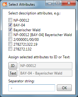
zone and the hemisphere. If an ArcView attribute file (.dbf) is
available, a window will open and show the attributes of the first
shape. The user may select the attributes which should be used to create
the sample ID and description. Check one or more appropriate boxes and
assign them by clicking the “ID” or “Text” button. A separator string
may be defined to combine the selected attributes to the final text
string. If no attribute is selected, the name of the ArcView file is
assigned to the sample description.
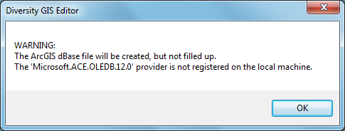
To access the dBase attributes file for reading or writing, the
Microsoft ACE OLEDB 12.0 driver must be installed on the computer. If it
is missing, the attributes cannot be evaluated and a warning will be
displayed. The shapes will be loaded properly, anyway, but no
description will be added.
When loading an image without world coordinates, it will be displayed
top left in the working area. If no background map is loaded yet, the
Screen symbol
 is shown in
the status line, followed by the screen coordinates of the current
cursor position.
is shown in
the status line, followed by the screen coordinates of the current
cursor position.
When loading an image with world coordinates and no background reference
map exists, it will be displayed top left in the working area. The World
symbol is
shown in the status line, followed by the screen coordinates and the
world coordinates of the current cursor position.
When loading an image with world coordinates having an existing
reference map, it will be embedded in the background map according to
its coordinates. If the new image does not overlap with the reference
map, the image exists virtually in the coordinate system, but possibly
could not be seen because it is too far away from the reference map.
Loaded images with world coordinates are immediately added to the Sample
List. When loading an image without world coordinates it is displayed,
but not yet added to the Sample List. The user has to add it manually by
pressing the Add button . This is because
the user should have the opportunity to adapt the image to the
background map to be stored later on with applicable coordinates.
GIS Editor
Save Samples
To save a background map which is currently displayed in Map mode just
press the Save button instead of the Add
button . A save file dialog will pop up to
name the file, the map and its coordinates will be saved and added to
the sample list.
A background map is required before objects and images can be saved.
Saving samples means saving their type, attributes and world coordinates
in files. When pressing the Save button ,
it applies to all visible samples on the working area, except the
background map. A current sample will be added to the sample list before
it is saved.
If objects are visible, a save file dialog will open and a name for the
target file(s) must be set. Objects (areas, line strings, points) will
be saved in respect to the selected formats of the GIS-EditorSettings:
- If MS-SQL is enabled, all visible objects will be collected and stored
in one GIS Editor shape file in text format (extension .shp1). The
file contains the objects’ attributes and MS-SQL Geo Object definition
strings. If altitude calculation is enabled in the GIS-Editor Settings, these values are stored, too.
- If ArcView is enabled, for each object 3 ArcView compatible shape
definition files in binary format will be created: A shape file, an
index file and a dBase file holding the description (extensions .shp,
.shx, .dbf).
If images are in the Sample List, they are already present on disk and
will not be saved twice. Instead for each image an XML file will be
created with the calculated world coordinates of the image and will be
stored under the same location and name as the image. This does not
apply to the current background map.
If Save Working Area is enabled in the GIS-EditorSettings, a scan of the complete working area
including its objects is made and stored in an image file, which name
has been set in the save file dialog.
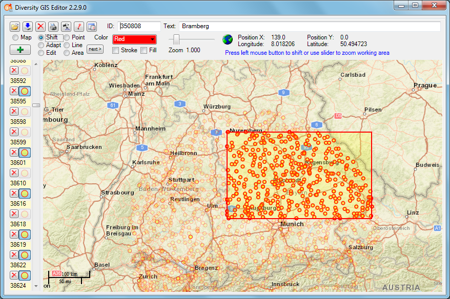
To save only a part of the working area the Frame box must be checked in
the GIS-Editor Settings, too. Then a
rectangular frame of the given dimensions is displayed, which defines
the part of the working area that will be saved. It can be dragged to
the right position using the left mouse button (click, hold and shift),
and it can be resized by grabbing and moving the corners of the frame.
GIS Editor
Delete Samples
To delete a single object of the Sample List just press the small Delete
button  left
of the Toggle button. The sample will be removed from the list and the
working area, the other sample entries will be rearranged.
left
of the Toggle button. The sample will be removed from the list and the
working area, the other sample entries will be rearranged.
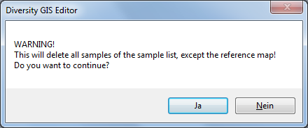
Pressing the large Delete button in the
Control Panel will remove all samples of the Sample List, except the
reference map. A warning is shown before:
GIS Editor
Print Samples
Pressing the Print button  in the Control
Panel will open a print dialog to select a printer and adjust the
settings. Then it will print the complete working area including all
visible objects. This feature is useful e.g. for documentations.
in the Control
Panel will open a print dialog to select a printer and adjust the
settings. Then it will print the complete working area including all
visible objects. This feature is useful e.g. for documentations.
GIS Editor
Settings
Pressing the Settings button  in the
Control Panel will open a dialog to adjust these GIS Editor settings
which are not frequently changed:
in the
Control Panel will open a dialog to adjust these GIS Editor settings
which are not frequently changed:
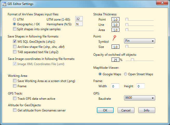
ArcView is a common Desktop GIS tool and stores its
data in binary files. The GIS Editor is able to read these files and
display the included geography objects. But because ArcView does not
necessarily provide a dedicated information about the GIS format of the
contained data, the user has to know and select it in advance.
The GIS Editor currently supports WGS84 geographic coordinates,
Gauß-Krüger coordinates (Potsdam datum) und WGS84 UTM coordinates. If
“Geographic / GK” is selected, the program will choose the right format
by checking the binary values. In case of UTM the user must select the
hemisphere (N/S) and the UTM zone (1-60) to ensure that the objects will
be displayed at the correct location.
The ArcView data files may contain complex geographic shapes (e.g.
polygons or line strings) which are combined by the GIS editor to one
multi object (e.g. multipolygon) by default. To split up the shapes into
single objects the option “Split shapes into single samples” has to be
selected. Then they are placed into the sample list separately. This
could be helpful to avoid out-of-memory errors if very large shapes
should be converted to SQL geography strings.
At the moment 3 formats for object files are supported:
- MS-SQL Geo Objects (.shp1)
- TAB separated text files (.shp2)
- ArcView shape files (.shp, .shx, .dbf)
Microsoft SQL Geo Objects are part of a standard for
storing geometry and geography data in an SQL database, as used by the
DiversityWorkbench modules. They are a well defined text string
containing the geometrical type (e.g. Polygon, Line, Point) and the
geographical coordinates (longitude, latitude, optional altitude) of an
object.
Together with the GIS Editor attributes (e.g. color, transparency) they
are stored in a proprietary GIS Editor shape file in ASCII text format.
This file can easily be read and changed using a text editor.
TAB separated text files are widely used as an interchange data file
format. The content of a file is more or less the same as above, but the
parameters of each object are placed in a single text line, separated by
tabulator characters. Additionally to the SQL Geo Object the “envelope
center point” (longitude and latitude) of it is saved separately in the
file.
The GIS Editor can also create ArcView compatible files to store the
samples, which then may be read from ArcView GIS tools. 3 files are
required for each type of shape: A data file with extension “.shp”, an
index file with extension “.shx” and a description file in dBase format
with extension “.dbf”.
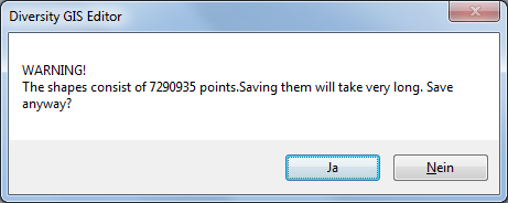
The advantage of the first format is the transparency and readability of
the data file, which is just one single text file. But storing huge
samples is time consuming, because they have to be converted to SQL
geography strings. If the samples consist of more than 100,000 points,
an warning message is shown and the user may decide whether to continue
or not:
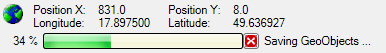
While saving the shapes, a progress bar will be displayed to indicate
the status of the task:
Using the ArcView format makes the data files compatible with many
applications. Huge samples can be stored much faster. But each type of
sample requires a separate set of output files, because different types
of objects within one file are not supported so far. So a sample list
containing 10 objects will produce 30 data files (file name with an
appended index, which is incremented for each sample). Furthermore the
attributes like color, transparency and stroke thickness will not be
saved.
Currently there is just one format supported for storing image
coordinates. They are written into an XML file which is also used in
DiversityMobile modules. Saving the coordinates in this format is
required for the GIS Editor, so it cannot be disabled.
Saving the working area
Selecting this check box and later on pressing the Save button
 will additionally scan the working area
including all visible objects and save it as an image file under the
name provided in the save file dialog, see SaveSamples. This is useful for documentations.
will additionally scan the working area
including all visible objects and save it as an image file under the
name provided in the save file dialog, see SaveSamples. This is useful for documentations.
Note: There are copyright restrictions on maps or aerial images
which are created with the Google maps viewer. Please contact Google
before using them for publications to grant a license, or use Open
Street Maps captures, which could be used freely under the
Creative Commons Attribution Share Alike license  conditions.
When checking the “Frame” box just a rectangular part of the working
area is saved. The size (in pixels) of the frame has to be defined in
the adjacent “Width” and “Height” fields. This is convenient if the
resulting image should have well defined dimensions, e.g. fit the
resolution of a smartphone display. After closing the Settings window a
rectangular frame of these dimensions is displayed on the working area
which defines the part to be saved. The frame is only visible in Shift
Mode. It can also be adjusted using the mouse: Place the cursor within
the frame, press the left mouse button und hold it, then shift the frame
by moving the mouse. Or change the size of the frame by grabbing a
corner: When the cursor changes, press the left mouse button und hold
it, then adjust the size by moving the mouse.
GPS Track
When checking this box the movement of the GPS marker on the background
map will be tracked by a line string. After switching off the GPS button
the line string will be added to the sample list automatically.
Altitude for geo objects
This box applies to MS-SQL Geo Objects only. If checked, the appropriate
altitude of the object points (longitude, latitude) will be stored in
the file, too. This is not recommended for sample objects with a lot of
points or vertices, because for every point the Geonames server has to
be contacted to request the associated altitude value. This could slow
down the saving procedure immensely.
Setting the stroke thickness
The stroke thickness for area, line strings and point symbols can be set
by using the appropriate slider. The value of the thickness is shown in
the label box left of the slider. Double clicking the slider will reset
the thickness to its default value 1.
Setting the Point symbol
The symbol for the points can be selected from the drop down menu. The
symbol size can be set using the slider below the menu. The point symbol
display will change accordingly.
Setting the opacity of switched off objects
The samples on the working area may be switched off and on with the
mouse buttons. If the switched off objects would become invisible, it
will be difficult to switch them on again, because you don’t see them.
For this the opacity of the switched off samples can be adjusted between
0% (invisible) and 100% (fully visible) with the slider. E.g. a value of
25% will make the samples transparent, but one can still see and touch
them on the map.
Setting the GPS baudrate
It is essential to set a suitable baudrate for a connected GPS device
according to its specification. The rate can be selected from the list
of the drop down menu. If no GPS device is available, Demo mode could be
chosen to see the behaviour of the functionality.
Setting the Map Mode viewer
The radio buttons offer the choice of the viewer for creating a
background map. Currently Google Maps and Open Street Maps are provided.
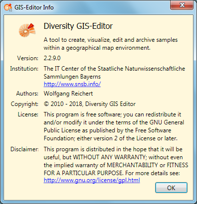
GIS Editor Info
Clicking the Info button will display a window containing GIS Editor
version and license information.
Saving the settings
Finally pressing the OK Button will save the settings, pressing the
Cancel button will discard them.
GIS Editor
Sample Detection
Since GIS Editor version 2.2.3.0 the Sample Detection offers a new
convenient tool to digitize sample markers e. g. of a scanned and
georeferenced analog paper sheet.
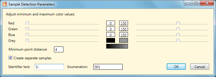
The tool will try to detect “points” on an image according to the
detection parameters which can be adjusted in the Sample Detection
Parameters window, which will open when clicking the
 button.
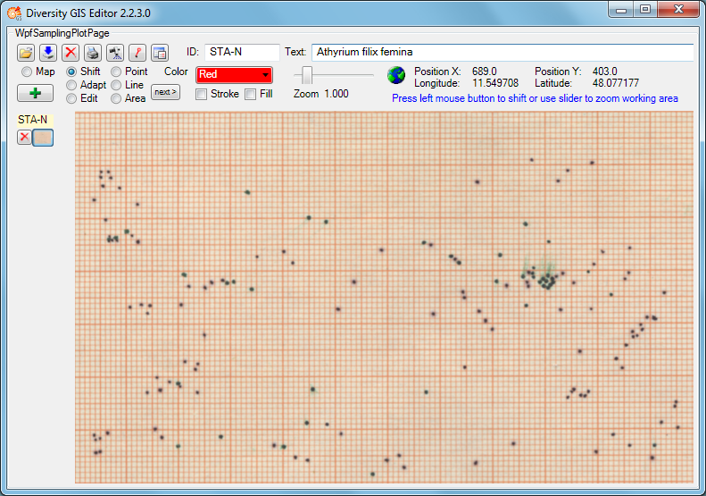
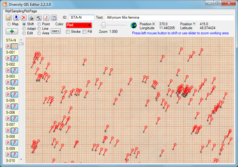
The decision what belongs to a sample and what is just background on the
loaded image is made by defining a color range of the object to be
found. Looking at the example picture above, we can see that the
collector has marked samples using a “black” pen on a reddish scale
paper. The points appear as dark grey scatterplots. To detect these
points we must define the color range of interest from “mid grey” to
“black”.
The grey range can be easily set by moving the “Grey” sliders for
minimum and maximum values. The sliders for the 3 color channels will
move simultaneously, adjusting the channel values in parallel. In the
example above we found a range from 0 (black) to 150 (mid grey) which
covers the colors of the samples and excludes the background colors. It
is visualized in the color boxes for min and max values and as a linear
gradient color brush.
If we’d look with a magnifying glass on a single point, we would
discover that in fact it is an array of pixels (picture elements) in
various shades of grey. To reduce this “cloud” to a single point
coordinate the program uses several algorithms. The result can be
improved by setting the parameter for the minimum point distance in
pixels to an appropriate value (e. g. 4).
The resulting sample points would be displayed as a point collection to
be (potentially) edited and added as one sample to the GIS Editor sample
list. In contrast, clicking the check box beneath will split up the
found sample points into single samples and add them immediately to the
sample list including an enumeration. The sample names will then be
composed by Identifier and Enumeration (start value, will be
incremented) as defined in the text boxes under it. Pressing the OK
button will start the detection and deliver the detected points as
object markers.
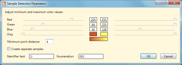
Not only grey points may be detected, but markers of any color tone. The
ranges for the red, green and blue color channels can be adjusted
individually by moving the sliders for min and max values. The gradient
color brush gives you a hint about the resulting color range, but it
needs much experience to define a color range properly to get the
expected results.

 or
or


 if an appropriate background map has
been loaded. If GPS Track in the
if an appropriate background map has
been loaded. If GPS Track in the